pylab command

'best' : 0,
'upper right' : 1, (default)
'upper left' : 2,
'lower left' : 3,
'lower right' : 4,
'right' : 5,
'center left' : 6,
'center right' : 7,
'lower center' : 8,
'upper center' : 9,
'center' : 10,

'lw' : 'linewidth'
'ls' : 'linestyle'
'c' : 'color'
'fc' : 'facecolor'
'ec' : 'edgecolor'
'mfc' : 'markerfacecolor'
'mec' : 'markeredgecolor'
'mew' : 'markeredgewidth'
'aa' : 'antialiased'

The following line styles are supported:
- : solid line
-- : dashed line
-. : dash-dot line
: : dotted line
. : points
, : pixels
o : circle symbols
^ : triangle up symbols
v : triangle down symbols
< : triangle left symbols
> : triangle right symbols
s : square symbols
+ : plus symbols
x : cross symbols
D : diamond symbols
d : thin diamond symbols
1 : tripod down symbols
2 : tripod up symbols
3 : tripod left symbols
4 : tripod right symbols
h : hexagon symbols
H : rotated hexagon symbols
p : pentagon symbols
| : vertical line symbols
_ : horizontal line symbols
steps : use gnuplot style 'steps' # kwarg only
The following color abbreviations are supported
b : blue
g : green
r : red
c : cyan
m : magenta
y : yellow
k : black
w : white

user webpage setting in apache2

It seems as though a recent update to the Apache2 package, upon a fresh install, renders the UserDir module not loaded by default. That is the ability to serve web pages from the ~/public_html directory on a per user basis.

Here's how to quickly enable this module at load time:

# a2enmod userdir
# /etc/init.d/apache2 force-reload

new monitor for debian

1. Hit Ctrl-Alt-F1 and login as root from the text console.
2. dpkg-reconfigure xserver-xfree86
3. When you get to the monitor config, you can either specify exact monitor frequencies with the "Advanced" setting or (I recommend) just specify the resolution and refresh rate you want X to use with the Normal settings control.
4. Save and logout
5. Ctrl-Alt-F7 to return to the GUI login
6. Hit Ctrl-Alt-Backspace to restart X with the new settings

configure a static IP in debian/redhat

To configure a static IP (an IP that will never change) in debian you must edit the file
/etc/networking/interfaces and put the following:

CODE

# /etc/network/interfaces -- configuration file for ifup(8), ifdown(8) # The loopback interface auto lo iface lo inet loopback # The first network card - this entry was created during the Debian installation # (network, broadcast and gateway are optional) auto eth0 iface eth0 inet static address 192.168.1.10 netmask 255.255.255.0 network 192.168.1.0 broadcast 192.168.1.255 gateway 192.168.1.1

The last section is the most important, the top may or may not be the same so don't play with it unless you get an error. In this case the IP of the server is 192.168.1.10 so if you run it as a DNS server for example, you can set that in your router's config and not worry about it changing.

To apply this configuration type /etc/init.d/networking restart

You'll get a message that it's restarting the network interface, then you'll get booted off ssh (because the IP changed) so reconnect using the new IP and it should work.

In red hat this file is /etc/sysconfig/network-scripts/ifcfg-eth0 and you would put this in it:

CODE

DEVICE=eth0 BOOTPROTO=static ONBOOT=yes IPADDR=192.168.1.10 NETMASK=255.255.255.0 GATEWAY=192.168.1.1

Cutting/pasting columns in Vim

In linux, ctrl -v for block select mode. use hjkl to select text. Edit/cut/past as usual.

In Ms Windows Ctrl - V is already assigned to paste. Vim for Windows uses
Ctrl-Q to start block select mode. You have to use the hjkl keys when
selecting text because the cursor keys simply drop you out of select mode.

Vim, making Windows almost bearable.

Scipy Fitting 2-D data

The data to be fitted is included in the file tgdata.dat and represents weight loss (in wt. %) as a function of time. The weight loss is due to hydrogen desorption from LiAlH₄, a potential material for on-board hydrogen storage in future fuel cell powered vehicles (thank you Ben for mentioning hydrogen power in the Laundrette in issue #114). The data is actually the same as in example 1 of LG#114. For some reason, I suspect that the data may be explained by the following function:

f(t) = A1*(1-exp(-(k1*t)^n1)) + A2*(1-exp(-(k2*t)^n2))

There are different mathematical methods available for finding the parameters that give an optimal fit to real data, but the most widely used is probably the Levenberg-Marquandt algorithm for non-linear least-squares optimization. The algorithm works by minimizing the sum of squares (squared residuals) defined for each data point as

(y-f(t))^2

where y is the measured dependent variable and f(t) is the calculated. The Scipy package has the Levenberg-Marquandt algorithm included as the function leastsq.

The fitting routine is in the file kinfit.py and the python code is listed below. Line numbers have been added for readability.

     1  from scipy import *
    2  from scipy.optimize import leastsq
    3  import scipy.io.array_import
    4  from scipy import gplt
    5
    6  def residuals(p, y, x):
    7          err = y-peval(x,p)
    8          return err
    9
   10  def peval(x, p):
   11          return p[0]*(1-exp(-(p[2]*x)**p[4])) + p[1]*(1-exp(-(p[3]*(x))**p[5] ))
   12
   13  filename=('tgdata.dat')
   14  data = scipy.io.array_import.read_array(filename)
   15
   16  y = data[:,1]
   17  x = data[:,0]
   18
   19  A1_0=4
   20  A2_0=3
   21  k1_0=0.5
   22  k2_0=0.04
   23  n1_0=2
   24  n2_0=1
   25  pname = (['A1','A2','k1','k2','n1','n2'])
   26  p0 = array([A1_0 , A2_0, k1_0, k2_0,n1_0,n2_0])
   27  plsq = leastsq(residuals, p0, args=(y, x), maxfev=2000)
   28  gplt.plot(x,y,'title "Meas" with points',x,peval(x,plsq[0]),'title "Fit" with lines lt -1')
   29  gplt.yaxis((0, 7))
   30  gplt.legend('right bottom Left')
   31  gplt.xtitle('Time [h]')
   32  gplt.ytitle('Hydrogen release [wt. %]')
   33  gplt.grid("off")
   34  gplt.output('kinfit.png','png medium transparent size 600,400')
   35
   36  print "Final parameters"
   37  for i in range(len(pname)):
   38          print "%s = %.4f " % (pname[i], p0[i])

In order to run the code download the kinfit.py.txt file as kinfit.py (or use another name of your preference), also download the datafile tgdata.dat and run the script with python kinfit.py. Besides Python, you need to have SciPy and gnuplot installed (vers. 4.0 was used throughout this article). The output of the program is plotted to the screen as shown below. A hard copy is also made. The gnuplot png option size is a little tricky. The example shown above works with gnuplot compiled against libgd. If you have libpng + zlib installed, instead of size write picsize and the specified width and height should not be comma separated. As shown in the figure below, the proposed model fit the data very well (sometimes you get lucky :-).

Now, let us go through the code of the example.

Line 1-4

all the needed packages are imported. The first is basic SciPy functionality, the second is the Levenberg-Marquandt algorithm, the third is ASCII data file import, and finally the fourth is the gnuplot interface.

Line 6-11

First, the function used to calculate the residuals (not the squared ones, squaring will be handled by leastsq) is defined; second, the fitting function is defined.

Line 13-17

The data file name is stored, and the data file is read using scipy.io.array_import.read_array. For convenience x (time) and y (weight loss) values are stores in separate variables.

Line 19-26

All parameters are given some initial guesses. An array with the names of the parameters is created for printing the results and all initial guesses are also stored in an array. I have chosen initial guesses that are quite close to the optimal parameters. However, chosing reasonable starting parameters is not always easy. In the worst case, poor initial parameters might result in the fitting procedure not being able to find a converged solution. In this case, a starting point can be to try and plot the data along with the model predictions and then "tune" the initial parameters to give just a crude description (but better than the initial parameters that did not lead to convergence), so that the model just captures the essential features of the data before starting the fitting procedure.

Line 27

Here the Levenberg-Marquandt algorithm (lestsq) is called. The input parameters are the name of the function defining the residuals, the array of initial guesses, the x- and y-values of the data, and the maximum number of function evaluation are also specified. The values of the optimized parameters are stored in plsq[0] (actually the initial guesses in p0 are also overwritten with the optimized ones). In order to learn more about the usage of lestsq type info(optimize.leastsq) in an interactive python session - remember that the SciPy package should be imported first - or read the tutorial (see references in the end of this article).

Line 28-34

This is the plotting of the data and the model calculations (by evaluating the function defining the fitting model with the final parameters as input).

Line 36-38

The final parameters are printed to the console as:

Final parameters

A1 = 4.1141

A2 = 2.4435

k1 = 0.6240

k2 = 0.1227

n1 = 1.7987

n2 = 1.5120

Gnuplot also uses the Levenberg-Marquandt algorithm for its built-in curve fitting procedure. Actually, for many cases where the fitting function is somewhat simple and the data does not need heavy pre-processing, I prefer gnuplot over Python - simply due to the fact that Gnuplot also prints standard error estimates of the individual parameters. The advantage of Python over Gnuplot is the availability of many different optimization algorithms in addition to the Levenberg-Marquandt procedure, e.g. the Simplex algorithm, the Powell's method, the Quasi-Newton method, Conjugated-gradient method, etc. One only has to supply a function calculating the sum of squares (with lestsq squaring and summing of the residuals were performed on-the-fly).

scipy spline example

# Cubic-spline
x = arange(0,2*pi+pi/4,2*pi/8)
y = sin(x)
tck = interpolate.splrep(x,y,s=0)
xnew = arange(0,2*pi,pi/50)
ynew = interpolate.splev(xnew,tck,der=0)
xplt.plot(x,y,’x’,xnew,ynew,xnew,sin(xnew),x,y,’b’)
xplt.legend([’Linear’,’Cubic Spline’, ’True’],[’b-x’,’m’,’r’])
xplt.limits(-0.05,6.33,-1.05,1.05)
xplt.title(’Cubic-spline interpolation’)
xplt.eps(’interp_cubic’)

# Derivative of spline
yder = interpolate.splev(xnew,tck,der=1)
xplt.plot(xnew,yder,xnew,cos(xnew),’|’)
xplt.legend([’Cubic Spline’, ’True’])
xplt.limits(-0.05,6.33,-1.05,1.05)
xplt.title(’Derivative estimation from spline’)
xplt.eps(’interp_cubic_der’)

# Integral of spline
def integ(x,tck,constant=-1):
x = asarray_1d(x)
out = zeros(x.shape, x.typecode())
for n in xrange(len(out)):
out[n] = interpolate.splint(0,x[n],tck)
out += constant
return out

yint = integ(xnew,tck)
xplt.plot(xnew,yint,xnew,-cos(xnew),’|’)
xplt.legend([’Cubic Spline’, ’True’])
xplt.limits(-0.05,6.33,-1.05,1.05)
xplt.title(’Integral estimation from spline’)
xplt.eps(’interp_cubic_int’)

# Roots of spline
print interpolate.sproot(tck)

# Parametric spline
t = arange(0,1.1,.1)
x = sin(2*pi*t)
y = cos(2*pi*t)
tck,u = interpolate.splprep([x,y],s=0)
unew = arange(0,1.01,0.01)
out = interpolate.splev(unew,tck)
xplt.plot(x,y,’x’,out[0],out[1],sin(2*pi*unew),cos(2*pi*unew),x,y,’b’)
xplt.legend([’Linear’,’Cubic Spline’, ’True’],[’b-x’,’m’,’r’])
xplt.limits(-1.05,1.05,-1.05,1.05)
xplt.title(’Spline of parametrically-defined curve’)
xplt.eps(’interp_cubic_param’)

(a) Cubic-spline (splrep)

(b) Derivative of spline (splev)

(c) Integral of spline (splint)

(d) Spline of parametric curve (splprep)

Figure 3:

Examples of using cubic-spline interpolation.

Firewalls with OpenSSH and PuTTY

I found this article is very useful. Copy and paste here for further reference. Qing

Breaking Firewalls with OpenSSH and PuTTY

If the system administrator deliberately filters out all traffic except port 22 (ssh), to a single server, it is very likely that you can still gain access other computers behind the firewall. This article shows how remote Linux and Windows users can gain access to firewalled samba, mail, and http servers. In essence, it shows how openSSH and PuTTY can be used as a VPN solution for your home or workplace, without monkeying with the firewall. This article is NOT suggesting you close port 22. These step are only possible given valid accounts on all servers. But, read on, you may be surprised what you can do, without punching additional holes through the firewall -- punching additional holes is a bad idea.

OpenSSH and Linux

From the Linux laptop 192.168.1.106, it is possible to get access to the resources behind the firewall directly, including SAMBA server, HTTP Server, and Mail Server which are blocked from the outside by the firewall. The firewall only permits access to the SSH Server via port 22; yet, as you will see, it is possible to get access to the other servers.

The SSH Server is seen as 66.35.250.203 from the outside. To tunnel traffic through the SSH Server, from the Linux laptop 192.168.1.106, create the following "~/.ssh/config" file, on the Linux laptop.

~/.ssh/config

## Linux Laptop .ssh/config ##
Host work
HostName 66.35.250.203
       User sporkey
       LocalForward 20000 192.168.0.66:80
       LocalForward 22000 192.168.0.66:22
       LocalForward 22139 192.168.0.8:139
       LocalForward 22110 192.168.0.5:110

Host http
HostName localhost
       User donkey
       Port 22000
       HostKeyAlias localhosthttp

This file must have the following rights.

  $  chmod 600 ~/.ssh/config

Take a look again at the file above. Note the entry for "LocalForward 22000 192.168.0.66:22", and compare this to the network diagram. The connection to the SSH Server is made by running the command below, from the Linux laptop (192.168.1.106).

 $ ssh -l sporkey 66.35.250.203

Quick hint: the above command can be shortened, since the user name "sporkey" and the "HostName" are already specified in the config file. Therefore, you can use "ssh work" as shown below.

 $ ssh work

After this connection is made, it is possible to access the HTTP Server directly, assuming the account donkey has access to this server. The following command below is executed on the Linux laptop (192.168.1.106). Yes, that is on the Linux laptop in a new window. Again, this will be executed from 192.168.1.106 in a new session. So note here the Linux laptop is getting direct access to (192.168.0.66). Reference the diagram above. This is the "localhost" of the Linux laptop -- you got this, right? The ssh sessions are initiated from the Linux laptop.

  $ ssh -l donkey localhost -p 22000

Since the config file maps "http" to localhost port 2200, the above command can be shortened to the following:

  $ ssh http

Wait, there is a better way. Instead of creating two terminal sessions, one for "ssh work", then, another one for "ssh http", why not put it all together in one command.

   $ ssh -N -f -q work;ssh http

The above command will establish the connection to work, forwarding the necessary ports to the other servers. The "-N" is for "Do not execute remote command", the "-f" requests ssh to go to the background, and "-q" is to suppress all warnings and diagnostic messages. So, still not short enough for you? Then create an alias, alias http='ssh -N -f -q work;ssh http' and put that in your "~.bashrc" file, which is about as short as you can get, since typing http on the command line would get you to the HTTP server.

To copy files to this server, the command below is used. Note uppercase "-P" follows "scp". If you are in the ".ssh" directory you will see an "authorized_keys2" and maybe an "authorized_keys", which you may want to append to the like files on the destination server. These files are only listed as an example. Any file could be copied; but, if you copy these files to the remote server and append the contents to the remote server's authorized_key* files, then, you will not be prompted for a password the next time you make a connection. See Tip 12 in Linux Tips. You will need to create an authorized_keys2 and authorized_keys file with all the public keys of the computers that will connect. Below, assume you have these keys in the currently directory on the laptop, and you want to copy this to the HTTP Sever [192.168.0.66]. The keys go in "~/.ssh/authorized_keys2" for ssh2. Again, take a look at Linux Tips . You do not want to write over any existing keys.

 $ scp -P 22000 authorized_keys* donkey@localhost:./.ssh/.

But, because you have everything in the "config" file, you can shorten the above command to the following:

 $ scp authorized_keys* http:./.ssh/.

The following command, executed from the Linux laptop, will download the web page from the remote server (192.168.0.66).

 $ wget http://localhost:20000/

Linux Laptop becomes Company Web Server -- Power of RemoteForward

Suppose the Linux laptop is running a web server. Is it possible for the people in the company to view this, the web server on the laptop (192.168.1.106), when they attach to HTTP Server (192.168.0.66)? Absolutely. Think about this because what is being suggested here is that a laptop, with no direct access to the HTTP server, is actually going to take over the company web server. Yes, that is exactly what will be shown here; although, instead of taking over the company web server, which is running on port 80 of (192.168.0.66), you will see how to add an additional web server on port 20080. However, if you are intent upon taking over the company web server, you would have to perform similar steps as root, since only root has the ability to take over the privileged ports. But, start with this example first, then, you'll see how to do this on port 80. To perform this magic, the "/etc/ssh/sshd_config", on the company web server (192.168.0.66), must have the variable "GatewayPorts" set to "yes", otherwise, only the users logged into HTTP Server will be able to see the laptop's web page. Instead, we want everyone in the company to have direct access to the added port.

 GatewayPorts yes

After making the change, you will need to restart sshd.

 $ /etc/init.d/sshd restart

In the Linux laptop's "~/.ssh/config" add the following entry RemoteForward 20080 localhost:80 so that the complete "~/.ssh/config" is shown below.

## Updated Linux Laptop .ssh/config  ##
Host work
HostName 66.35.250.203
       User sporkey
       LocalForward 20000 192.168.0.66:80
       LocalForward 22000 192.168.0.66:22
       LocalForward 22139 192.168.0.8:139
       LocalForward 22110 192.168.0.5:110

Host http
HostName localhost
       User donkey
       Port 22000 
       RemoteForward 20080 localhost:80
       HostKeyAlias localhosthttp

If you perform a "netstat -l" from 192.168.0.66, the remote company web server, you should see the following:

 tcp  0  0 *:20080 *:*  LISTEN

This means that anyone, in the company, can view this webpage http://192.168.0.66:20080/ on port 20080. If you wanted port 80, the default http port, the connected user would have to have root privileges.

If you did not change the "/etc/ssh/sshd_config" file, "GatewayPorts" defaults to "no". And executing a "netstat -l" (that's an ell), would return the following:

 tcp   0 0 ::1:20080 *:* LISTEN

With the above restrictions, only users on the computer 192.168.0.66 would see the webpage on 192.168.1.106 from port 20080. This is what happens by default, since "GatewayPorts" is set to no.

By the way, did you figure out what the HostKeyAlias command does? If you make multiple localhost entries in your config file without HostKeyAlias, .ssh/known_hosts will contain multiple entries for "localhost" with different keys. Try it without HostKeyAlias and it should bark at you.

For references on generating ssh key pairs, securing an ssh server from remote root access, and samba mounts through an ssh tunnel see (TIP 12, TIP 13, and TIP 138) in Linux Tips listed at the end of this article. In addition,if you are a system administrator, may want to take note of (TIP 14), keeping yearly logs, and (TIP 26), which shows how to kill a user and all their running processes. In addition, the following (TIP 10, TIP 11, TIP 15, TIP 24, TIP 47, TIP 52, TIP 89, TIP 104, TIP 148, and TIP 150) may help with system security.

PuTTY for WindowsXP

From your Windows XP laptop, you want access to the following resources behind a firewall "SSH server", "Mail Server", and "HTTP Server". The only port allowed in is ssh, port 22, to the "SSH Server". So, how do you get access, from the laptop to the other resources using an ssh tunnel?

Step 1: (Download PuTTY)

Download putty.exe and plink.exe. Although plink.exe is not needed, it provides some handy features you may end up using later.

I normally put the files in "c:/bin", then, add this directory to the path.

Step 2: (Load the IP Address of Your Server)

Substitute the IP address 66.35.250.203 for the IP address of your ssh server and save it. Note 66.35.250.203 really is sourceforge, so unless you're access projects on sourceforge, you probably want a different IP address.

Step 3: (Create the Necessary Tunnels)

There are 2 additional servers you need access to. The "HTTP server" 192.168.0.66, and "Mail server" 192.168.0.5. Click on Tunnel and fill in the following values. The HTTP server works on port 80, so enter 80 in the Source port. The destination is 192.168.0.60:80. Hit "Add" to commit this entry.

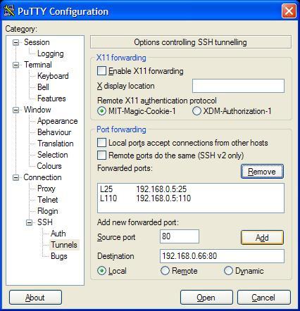
Your listing should be similar to the following. Make sure each entry has an "L" listed in front of it. Local port 25 will now go to server 192.168.0.5 on port 25. But, ports 110 and 25 will go to server 192.168.0.5.

Step 4: (Testing the Connection)

If you now open your ssh connection, click on "Sourceforge", or whatever you name it, then, you can browse the data on the "HTTP Server" by filling in local host at the browser. It makes sense to "Check" the connection at this stage -- remember to put in the correct IP addresses for your server.

Step 5: (Setting up Mail)

Mozilla Thunderbird is an excellent mail package. It will work in place of Microsoft Outlook, when connect to your work's Exchange, Postfix, or Sendmail server.

The server location is localhost. And notice the option below to "Leave messages on server". If you have another email client on your workstation at work, then, you might want to keep the mail on the server.

Step 6: (Getting Access to Samba Shares -- Loopback Adapter)

From the Windows XP computer, you want to add a Micosoft loopback Adapter. From the control panel, follow the steps below. By the way, it is possible to add more than one adapter.

  1.  Yes, I already connected the hardware
 2.  Add a new hardware device (bottom of menu)
 3.  Install the hardware that I manually select from a list (Advanced)
 4.  Select Network Adapters
 5.  Micosoft Loopback Adapter

Once the adapter is added, you must assign an IP address. The first adapter will be assigned 10.0.0.1, the second will be assigned 10.0.0.2, etc. DO NOT enter a "Default gateway".

The second adapter will have the IP address 10.0.0.2. Remember, there are two samba servers in the network diagram. Both the HTTP server and the SAMBA server have samba shares. Again, DO NOT enter a "Default gateway".

The loopback Adapters should appear in the control panel

Step 7: (Getting Access to Samba Shares -- SSH Configuration Settings)

Now you want to go back into the Putty configuration. In the "Source port" text box, yes it is small, enter 10.0.0.1:139; but note, the image below only shows 0.0.1:139 because it has scrolled to the left. Also, enter 192.168.0.66:139 for the destination address. When done, click "Add".

The completed entry should look like the following:

You can repeat the same procedure above for more samba shares, if you want. Although not shown, the same procedure is used for 10.0.0.2:139; but, it will have a destination of 192.168.0.8. Again, there are two samba shares in the network diagram.

Step 8: (Getting Access to Samba Shares -- View It)

To view the samba share, click Start/Run and type in \\10.0.0.1\

Special Note

You will probably have to reboot. Also, read and download the following patch from Microsoft.

Also, disable File and Printer Sharing for Microsoft Networks for both adapters.

Disable NetBIOS over TCP/IP; but, make sure LMHosts Lookup is enabled.

DOWNLOADS

OpenSSH
www.openssh.org

PuTTY
http://www.chiark.greenend.org.uk/~sgtatham/putty/download.html

ADDITIONAL TUTORIALS

Linux System Admin Tips There are over 200 Linux tips and tricks in this article. That is over 150 pages covering topics from setting and keeping the correct time on your computer, permanently deleting documents with shred, making files "immutable" so that root cannot change or delete, setting up more than one IP address on a single NIC, monitering users and processes, setting log rotate to monthly with 12 months of backups in compressed format, creating passwords for Apache using the htpasswd command, common Perl commands, using cfengine, adding users to groups, finding out which commands are aliased, query program text segment size and data segment size, trusted X11 forwarding, getting information on the hard drive including the current temperature, using Gnuplot, POVRAY and making animated GIFs, monitoring selective traffic with tcpdump and netstat, multiple examples using the find command, getting the most from Bash, plus a lot more. You can also down this article as a text document here for easy grepping.

Linux Quota Tutorial This tutorial walks you through implementing disk quotas for both users and groups on Linux, using a virtual filesystem, which is a filesystem created from a disk file. Since quotas work on a per-filesystem basis, this is a way to implement quotas on a sub-section, or even multiple subsections of your drive, without reformatting. This tutorial also covers quotactl, or quota's C interface, by way of an example program that can store disk usage in a SQLite database for monitoring data usage over time.

Google Gmail on Home Linux Box using Postfix and Fetchmail If you have a Google Gmail account, you can relay mail from your home linux system. It's a good exercise in configuring Postfix with TLS and SASL. Plus, you will learn how to bring down the mail safely, using fetchmail with the "sslcertck" option, that is, after you have verify and copied the necessary certificates. You'll learn it all from this tutorial. And you'll have Gmail running on your local Postfix MTA.

Create your own custom Live Linux CD These steps will show you how to create a functioning Linux system, with the latest 2.6 kernel compiled from source, and how to integrate the BusyBox utilities including the installation of DHCP. Plus, how to compile in the OpenSSH package on this CD based system. On system boot-up a filesystem will be created and the contents from the CD will be uncompressed and completely loaded into RAM -- the CD could be removed at this point for boot-up on a second computer. The remaining functioning system will have full ssh capabilities. You can take over any PC assuming, of course, you have configured the kernel with the appropriate drivers and the PC can boot from a CD.

MySQL Tips and Tricks Find out who is doing what in MySQL and how to kill the process, create binary log files, connect, create and select with Perl and Java, remove duplicates in a table with the index command, rollback and how to apply, merging several tables into one, updating foreign keys, monitor port 3306 with the tcpdump command, creating a C API, XML and HTML output, spatial extensions, complex selects, and much more.

SQLite Tutorial This article explores the power and simplicity of sqlite3, first by starting with common commands and triggers, then the attach statement with the union operation is introduced in a way that allows multiple tables, in separate databases, to be combined as one virtual table, without the overhead of copying or moving data. Next, the simple sign function and the amazingly powerful trick of using this function in SQL select statements to solve complex queries with a single pass through the data is demonstrated, after making a brief mathematical case for how the sign function defines the absolute value and IF conditions.

Lemon Parser Tutorial Lemon is a compact, thread safe, well-tested parser generator written by D. Richard Hipp. Using a parser generator, along with a scanner like flex, can be advantageous because there is less code to write. You just write the grammar for the parser. This article is an introduction to the Lemon Parser, complete with examples.

Errata

Special thanks to the following people who pointed out needed corrections.

[Sun Oct 9 13:32:01 EDT 2005] Kent West

---

Mike Chirico, a father of triplets (all girls) lives outside of Philadelphia, PA, USA. He has worked with Linux since 1996, has a Masters in Computer Science and Mathematics from Villanova University, and has worked in computer-related jobs from Wall Street to the University of Pennsylvania. His hero is Paul Erdos, a brilliant number theorist who was known for his open collaboration with others.

Mike's notes page is souptonuts. For open source consulting needs, please send an email to mchirico@comcast.net. All consulting work must include a donation to SourceForge.net.

Cubic spline (Python)

class Interpolator:
   def __init__(self, name, func, points, deriv=None):
       self.name = name  # used for naming the C function
       self.intervals = intervals = [ ]
       # Generate a cubic spline for each interpolation interval.
       for u, v in map(None, points[:-1], points[1:]):
           FU, FV = func(u), func(v)
           # adjust h as needed, or pass in a derivative function
           if deriv == None:
               h = 0.01
               DU = (func(u + h) - FU) / h
               DV = (func(v + h) - FV) / h
           else:
               DU = deriv(u)
               DV = deriv(v)
           denom = (u - v)**3
           A = ((-DV - DU) * v + (DV + DU) * u +
                2 * FV - 2 * FU) / denom
           B = -((-DV - 2 * DU) * v**2  +
                 u * ((DU - DV) * v + 3 * FV - 3 * FU) +
                 3 * FV * v - 3 * FU * v +
                 (2 * DV + DU) * u**2) / denom
           C = (- DU * v**3  +
                u * ((- 2 * DV - DU) * v**2  + 6 * FV * v
                                   - 6 * FU * v) +
                (DV + 2 * DU) * u**2 * v + DV * u**3) / denom
           D = -(u *(-DU * v**3  - 3 * FU * v**2) +
                 FU * v**3 + u**2 * ((DU - DV) * v**2 + 3 * FV * v) +
                 u**3 * (DV * v - FV)) / denom
           intervals.append((u, A, B, C, D))

   def __call__(self, x):
       def getInterval(x, intervalList):
           # run-time proportional to the log of the length
           # of the interval list
           n = len(intervalList)
           if n < 2:
               return intervalList[0]
           n2 = n / 2
           if x < intervalList[n2][0]:
               return getInterval(x, intervalList[:n2])
           else:
               return getInterval(x, intervalList[n2:])
       # Tree-search the intervals to get coefficients.
       u, A, B, C, D = getInterval(x, self.intervals)
       # Plug coefficients into polynomial.
       return ((A * x + B) * x + C) * x + D

   def c_code(self):
       """Generate C code to efficiently implement this
       interpolator. Run the C code through 'indent' if you
       need it to be legible."""
       def codeChoice(intervalList):
           n = len(intervalList)
           if n < 2:
               return ("A=%.10e;B=%.10e;C=%.10e;D=%.10e;"
                       % intervalList[0][1:])
           n2 = n / 2
           return ("if (x < %.10e) {%s} else {%s}"
                   % (intervalList[n2][0],
                      codeChoice(intervalList[:n2]),
                      codeChoice(intervalList[n2:])))
       return ("double interpolator_%s(double x) {" % self.name +
               "double A,B,C,D;%s" % codeChoice(self.intervals) +
               "return ((A * x + B) * x + C) * x + D;}")

TDerivative for excel

The following script will take the derivative of all the plotted datasets in the active graph window. It assumes that these datasets all share the same X values. It then stores the derivative datasets in one new worksheet, named TDerivative.

%W=%H;  //store the name of the active window

layer -c; //count stores the number of plotted datasets and %Z stores concatenated names of datasets

GetEnumWks TDerivative; //open new wks and name it TDerivative

copy -x %[%Z,#1] %(%H,2); //copy datasets to the new wks

deriv %(%H,2); //take the derivative of these datasets

wks.col2.label$="Derivative of %[%Z,#1]";

loop(ii,2,count){

wks.addcol();

%(%H,ii+1)=%[%Z,#ii];

deriv %(%H,ii+1); 

wks.col$(ii+1).label$="Derivative of %[%Z,#ii]";

}

wks.labels();