write example for fortran 90

WRITE(*,*) itest ! 1234567
WRITE(*,'(I6)') itest ! ******
WRITE(*,'(I10)') itest ! 1234567
WRITE(*,'(I10.9)') itest ! 001234567
WRITE(*,'(2I7)') itest, 7654321 ! 12345677654321
WRITE(*,'(2I8)') itest, 7654321 ! 1234567 7654321

WRITE(*,*) itest ! 1.2345670E+02 -not F format
WRITE(*,'(F8.0)') itest ! 123
WRITE(*,'(F10.4)') itest ! 123.4567
WRITE(*,'(F10.5)') itest ! 123.45670
WRITE(*,'(F10.9)') itest ! **********
WRITE(*,'(2F8.4)') itest, 7654321 ! 123.4567765.4321
WRITE(*,'(2F10.4)') itest, 7654321 ! 123.4567 765.4321

WRITE(*,*) itest ! 1.2345670E+02
WRITE(*,'(E10.4)') itest ! 0.1234E+09
WRITE(*,'(E10.5)') itest ! .12345E+09
WRITE(*,'(E10.4E3)') itest ! .1234E+009
WRITE(*,'(E10.9)') itest ! **********
WRITE(*,'(2E12.4)') itest, 7654321 ! 0.12345E+090.76543E+04
WRITE(*,'(2E10.4)') itest, 7654321 ! 0.1234E+090.7654E+04

WRITE(*,*) itest ! 1.2345000E+04
WRITE(*,'(EN13.6)') ! 12.345000E+03
WRITE(*,'(ES13.6)') ! 1.234500E+04 ES - Scientific - the value before the decimal point always lies in the range 1..10

CHARACTER(LEN=8) :: long='Bookshop'
CHARACTER(LEN=1) :: short='B'
WRITE(*,*) long ! Bookshop
WRITE(*,'(A)') long ! Bookshop
WRITE(*,'(A8)') long ! Bookshop
WRITE(*,'(A5)') long ! Books
WRITE(*,'(A10)') long ! Bookshop
WRITE(*,'(A)') short ! B
WRITE(*,'(2A) short, long ! BBookshop
WRITE(*,'(2A3) short, long ! BBoo

LOGICAL :: ltest=.FALSE.
WRITE(*,*) ltest ! F
WRITE(*,'(2L1)') ltest, .NOT.ltest ! FT
WRITE(*,'(L7)') ltest ! F

WRITE(*,'(I4, 2X, I4)') i, i-1 ! 1234 1233 Blank Spaces (Skip Character Positions)
WRITE(*,'(I4, 4X, I4)') i, i-1 ! 1234 1233

Special Characters

' ' to output the character string specified
/ specifies take a new line
( ) to group descriptors, normally for repetition
INTEGER :: value = 100
INTEGER :: a=101, b=201
WRITE(*,'( 'The value is', 2X, I3, ' units.')') value
WRITE(*,'( 'a =', 1X, I3, /, 'b = ', 1X, I3)')
WRITE(*,'( 'a and b =', 2(1X, I3) )') a, b

pylab command

'best' : 0,
'upper right' : 1, (default)
'upper left' : 2,
'lower left' : 3,
'lower right' : 4,
'right' : 5,
'center left' : 6,
'center right' : 7,
'lower center' : 8,
'upper center' : 9,
'center' : 10,

'lw' : 'linewidth'
'ls' : 'linestyle'
'c' : 'color'
'fc' : 'facecolor'
'ec' : 'edgecolor'
'mfc' : 'markerfacecolor'
'mec' : 'markeredgecolor'
'mew' : 'markeredgewidth'
'aa' : 'antialiased'

The following line styles are supported:
- : solid line
-- : dashed line
-. : dash-dot line
: : dotted line
. : points
, : pixels
o : circle symbols
^ : triangle up symbols
v : triangle down symbols
< : triangle left symbols
> : triangle right symbols
s : square symbols
+ : plus symbols
x : cross symbols
D : diamond symbols
d : thin diamond symbols
1 : tripod down symbols
2 : tripod up symbols
3 : tripod left symbols
4 : tripod right symbols
h : hexagon symbols
H : rotated hexagon symbols
p : pentagon symbols
| : vertical line symbols
_ : horizontal line symbols
steps : use gnuplot style 'steps' # kwarg only
The following color abbreviations are supported
b : blue
g : green
r : red
c : cyan
m : magenta
y : yellow
k : black
w : white

user webpage setting in apache2

It seems as though a recent update to the Apache2 package, upon a fresh install, renders the UserDir module not loaded by default. That is the ability to serve web pages from the ~/public_html directory on a per user basis.

Here's how to quickly enable this module at load time:

# a2enmod userdir
# /etc/init.d/apache2 force-reload

new monitor for debian

1. Hit Ctrl-Alt-F1 and login as root from the text console.
2. dpkg-reconfigure xserver-xfree86
3. When you get to the monitor config, you can either specify exact monitor frequencies with the "Advanced" setting or (I recommend) just specify the resolution and refresh rate you want X to use with the Normal settings control.
4. Save and logout
5. Ctrl-Alt-F7 to return to the GUI login
6. Hit Ctrl-Alt-Backspace to restart X with the new settings

configure a static IP in debian/redhat

To configure a static IP (an IP that will never change) in debian you must edit the file
/etc/networking/interfaces and put the following:

CODE

# /etc/network/interfaces -- configuration file for ifup(8), ifdown(8) # The loopback interface auto lo iface lo inet loopback # The first network card - this entry was created during the Debian installation # (network, broadcast and gateway are optional) auto eth0 iface eth0 inet static address 192.168.1.10 netmask 255.255.255.0 network 192.168.1.0 broadcast 192.168.1.255 gateway 192.168.1.1

The last section is the most important, the top may or may not be the same so don't play with it unless you get an error. In this case the IP of the server is 192.168.1.10 so if you run it as a DNS server for example, you can set that in your router's config and not worry about it changing.

To apply this configuration type /etc/init.d/networking restart

You'll get a message that it's restarting the network interface, then you'll get booted off ssh (because the IP changed) so reconnect using the new IP and it should work.

In red hat this file is /etc/sysconfig/network-scripts/ifcfg-eth0 and you would put this in it:

CODE

DEVICE=eth0 BOOTPROTO=static ONBOOT=yes IPADDR=192.168.1.10 NETMASK=255.255.255.0 GATEWAY=192.168.1.1

Cutting/pasting columns in Vim

In linux, ctrl -v for block select mode. use hjkl to select text. Edit/cut/past as usual.

In Ms Windows Ctrl - V is already assigned to paste. Vim for Windows uses
Ctrl-Q to start block select mode. You have to use the hjkl keys when
selecting text because the cursor keys simply drop you out of select mode.

Vim, making Windows almost bearable.

Scipy Fitting 2-D data

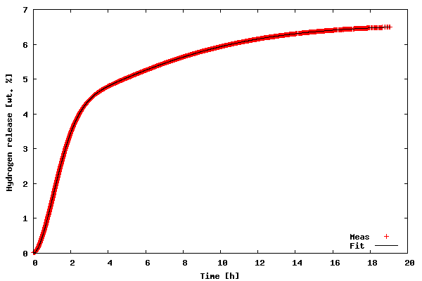
The data to be fitted is included in the file tgdata.dat and represents weight loss (in wt. %) as a function of time. The weight loss is due to hydrogen desorption from LiAlH₄, a potential material for on-board hydrogen storage in future fuel cell powered vehicles (thank you Ben for mentioning hydrogen power in the Laundrette in issue #114). The data is actually the same as in example 1 of LG#114. For some reason, I suspect that the data may be explained by the following function:

f(t) = A1*(1-exp(-(k1*t)^n1)) + A2*(1-exp(-(k2*t)^n2))

There are different mathematical methods available for finding the parameters that give an optimal fit to real data, but the most widely used is probably the Levenberg-Marquandt algorithm for non-linear least-squares optimization. The algorithm works by minimizing the sum of squares (squared residuals) defined for each data point as

(y-f(t))^2

where y is the measured dependent variable and f(t) is the calculated. The Scipy package has the Levenberg-Marquandt algorithm included as the function leastsq.

The fitting routine is in the file kinfit.py and the python code is listed below. Line numbers have been added for readability.

     1  from scipy import *
    2  from scipy.optimize import leastsq
    3  import scipy.io.array_import
    4  from scipy import gplt
    5
    6  def residuals(p, y, x):
    7          err = y-peval(x,p)
    8          return err
    9
   10  def peval(x, p):
   11          return p[0]*(1-exp(-(p[2]*x)**p[4])) + p[1]*(1-exp(-(p[3]*(x))**p[5] ))
   12
   13  filename=('tgdata.dat')
   14  data = scipy.io.array_import.read_array(filename)
   15
   16  y = data[:,1]
   17  x = data[:,0]
   18
   19  A1_0=4
   20  A2_0=3
   21  k1_0=0.5
   22  k2_0=0.04
   23  n1_0=2
   24  n2_0=1
   25  pname = (['A1','A2','k1','k2','n1','n2'])
   26  p0 = array([A1_0 , A2_0, k1_0, k2_0,n1_0,n2_0])
   27  plsq = leastsq(residuals, p0, args=(y, x), maxfev=2000)
   28  gplt.plot(x,y,'title "Meas" with points',x,peval(x,plsq[0]),'title "Fit" with lines lt -1')
   29  gplt.yaxis((0, 7))
   30  gplt.legend('right bottom Left')
   31  gplt.xtitle('Time [h]')
   32  gplt.ytitle('Hydrogen release [wt. %]')
   33  gplt.grid("off")
   34  gplt.output('kinfit.png','png medium transparent size 600,400')
   35
   36  print "Final parameters"
   37  for i in range(len(pname)):
   38          print "%s = %.4f " % (pname[i], p0[i])

In order to run the code download the kinfit.py.txt file as kinfit.py (or use another name of your preference), also download the datafile tgdata.dat and run the script with python kinfit.py. Besides Python, you need to have SciPy and gnuplot installed (vers. 4.0 was used throughout this article). The output of the program is plotted to the screen as shown below. A hard copy is also made. The gnuplot png option size is a little tricky. The example shown above works with gnuplot compiled against libgd. If you have libpng + zlib installed, instead of size write picsize and the specified width and height should not be comma separated. As shown in the figure below, the proposed model fit the data very well (sometimes you get lucky :-).

Now, let us go through the code of the example.

Line 1-4

all the needed packages are imported. The first is basic SciPy functionality, the second is the Levenberg-Marquandt algorithm, the third is ASCII data file import, and finally the fourth is the gnuplot interface.

Line 6-11

First, the function used to calculate the residuals (not the squared ones, squaring will be handled by leastsq) is defined; second, the fitting function is defined.

Line 13-17

The data file name is stored, and the data file is read using scipy.io.array_import.read_array. For convenience x (time) and y (weight loss) values are stores in separate variables.

Line 19-26

All parameters are given some initial guesses. An array with the names of the parameters is created for printing the results and all initial guesses are also stored in an array. I have chosen initial guesses that are quite close to the optimal parameters. However, chosing reasonable starting parameters is not always easy. In the worst case, poor initial parameters might result in the fitting procedure not being able to find a converged solution. In this case, a starting point can be to try and plot the data along with the model predictions and then "tune" the initial parameters to give just a crude description (but better than the initial parameters that did not lead to convergence), so that the model just captures the essential features of the data before starting the fitting procedure.

Line 27

Here the Levenberg-Marquandt algorithm (lestsq) is called. The input parameters are the name of the function defining the residuals, the array of initial guesses, the x- and y-values of the data, and the maximum number of function evaluation are also specified. The values of the optimized parameters are stored in plsq[0] (actually the initial guesses in p0 are also overwritten with the optimized ones). In order to learn more about the usage of lestsq type info(optimize.leastsq) in an interactive python session - remember that the SciPy package should be imported first - or read the tutorial (see references in the end of this article).

Line 28-34

This is the plotting of the data and the model calculations (by evaluating the function defining the fitting model with the final parameters as input).

Line 36-38

The final parameters are printed to the console as:

Final parameters

A1 = 4.1141

A2 = 2.4435

k1 = 0.6240

k2 = 0.1227

n1 = 1.7987

n2 = 1.5120

Gnuplot also uses the Levenberg-Marquandt algorithm for its built-in curve fitting procedure. Actually, for many cases where the fitting function is somewhat simple and the data does not need heavy pre-processing, I prefer gnuplot over Python - simply due to the fact that Gnuplot also prints standard error estimates of the individual parameters. The advantage of Python over Gnuplot is the availability of many different optimization algorithms in addition to the Levenberg-Marquandt procedure, e.g. the Simplex algorithm, the Powell's method, the Quasi-Newton method, Conjugated-gradient method, etc. One only has to supply a function calculating the sum of squares (with lestsq squaring and summing of the residuals were performed on-the-fly).